Feature Transformation
Any machine learning model must have a solid feature space, which is a fundamental need. Unfortunately, it is frequently unclear which attribute is more crucial. Because of this, all of the data set's qualities are employed as features, and the learning model is tasked with selecting the most crucial ones. This approach is absolutely not workable, especially for some domains, such as text classification, medical picture classification, etc. We can express a document as a bag of words if a model needs to be trained to determine if it is spam or not. Then, all distinct terms that appear in all documents will be included in the feature space. This feature space should have a few hundred thousand features. The number of features will reach millions if bigrams or trigrams are added to the list of features along with words. The use of feature transformation is made in order to solve this issue.
The performance of learning models is improved by dimensionality reduction techniques such as feature transformation.
The two main objectives of feature transformation are as follows:
-
Achieving best reconstruction of the original features in the data set
-
Achieving highest efficiency in the learning task
Feature Construction
Feature construction involves transforming a given set of input features to generate a new set of more powerful features. To understand more clearly, let's take the example of a real estate data set having details of all apartments sold in a specific region.
The data set has three features —apartment length, apartment breadth, and price of the apartment. Such data can serve as training data for the regression model if it is utilised as an input to a regression problem. The model should therefore be able to estimate the price of an apartment whose price is unknown or which has recently gone up for sale given the training data. The area of the apartment, which is not a component of the data set, is far more practical and makes more sense than utilising the length and width of the flat as a predictor. As a result, the data set can now include such a feature, namely apartment area. In other words, we add the newly "found" feature apartment area to the original data set and convert the three-dimensional data set to a four-dimensional data set.
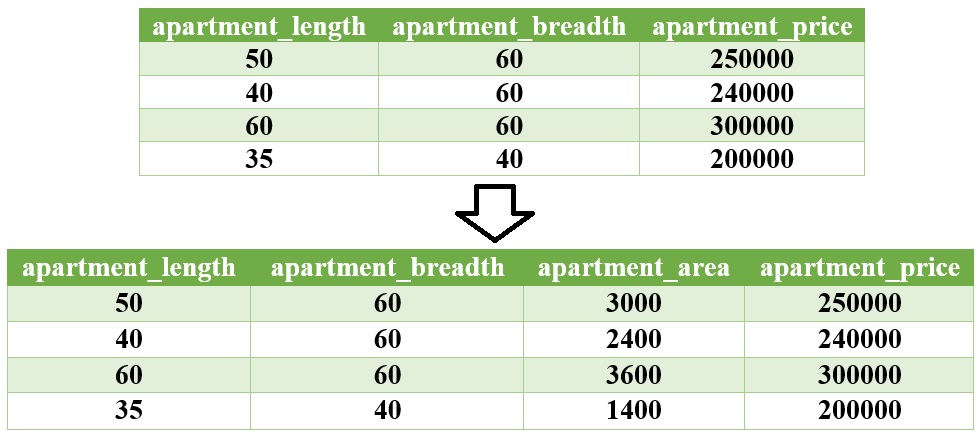
Figure: Feature construction
Feature Extraction
New features are produced through the combination of original features in feature extraction. Some of the commonly used operators for combining the original features include
- For Boolean features: Conjunctions, Disjunctions, Negation, etc.
- For nominal features: Cartesian product, M of N, etc.
- For numerical features: Min, Max, Addition, Subtraction, Multiplication, Division, Average, Equivalence, Inequality, etc.
Feature Extraction Algorithms
Most popular feature extraction algorithms used in machine learning:
Principal Component Analysis
Every data set, as we have seen, has multiple attributes or dimensions —many of which might have similarity with each other. For example, a person's height and weight tend to be fairly correlated. In general, weight and height are inversely correlated. So, it makes sense to expect a high degree of similarity between height and weight if those two attributes are included in a data set. Any machine learning algorithm, in general, performs better the fewer related attributes or features there are. In other words, the fact that there aren't many features and that they have little in common with one another is crucial to machine learning's success. This is the principal guiding principle of the feature extraction method known as principal component analysis (PCA).
In PCA, a new set of features that are quite different from the original features are extracted. As a result, an m-dimensional feature space is transformed into an m-dimensional feature space in which the dimensions are orthogonal, or wholly unrelated to one another. We must take a step back and do a superficial dive into the vector space concept in linear algebra in order to understand the concept of orthogonality.
We all know that a vector is a quantity having both magnitude and direction and hence can determine the position of a point relative to another point in the Euclidean space (i.e. a two or three or 'n' dimensional space). A vector space is a set of vectors. Vector spaces have a property that they can be represented as a linear combination of a smaller set of vectors, called basis vectors. So, any vector 'v' in a vector space can be represented as
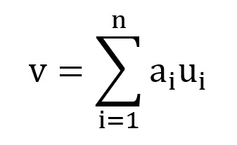
where, ai represents 'n' scalars and represents the basis vectors. Basis vectors are orthogonal to each other. Orthogonality of vectors in n-dimensional vector space can be thought of an extension of the vectors being perpendicular in a two-dimensional vector space. Two orthogonal vectors are completely unrelated or independent of each other. So the transformation of a set of vectors to the corresponding set of basis vectors such that each vector in the original set can be expressed as a linear combination of basis vectors helps in decomposing the vectors to a number of independent components.
The objective of PCA is to make the transformation in such a way that
1: The new features are distinct, i.e. the covariance between the new features, i.e. the principal components is 0,
2: The order in which the principal components are produced reflects how variable the data it captures is. Because of this, the first principal component should capture the highest level of variability, the second principal component should capture the next-highest level of variability, etc.
3: The sum of variance of the new features or the principal components should be equal to the sum of variance of the original features
PCA works based on a process called eigenvalue decomposition of a covariance matrix of a data set. Below are the steps to be followed:
-
First, calculate the covariance matrix of a data set.
-
Then, calculate the eigenvalues of the covariance matrix.
-
The eigenvector having highest eigenvalue represents the direction in which there is the highest variance. So this will help in identifying the first principal component.
-
The eigenvector having the next highest eigenvalue represents the direction in which data has the highest remaining variance and also orthogonal to the first direction. So, this helps in identifying the second principal component.
Like this, identify the top 'k' eigenvectors having top 'k' eigenvalues so as to get the 'k' principal components.
Singular Value Decomposition
Singular value decomposition (SVD) is a matrix factorization technique commonly used in linear algebra. SVD of a matrix A (m x n) is a factorization of the form:
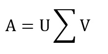
where is a m x n rectangular diagonal matrix, U and V are orthonormal matrices, U is a m x m unitary matrix, V is a n x n unitary matrix, and the singular values of matrix A are the diagonal entries of ∑. The left-singular and right-singular vectors of matrix A are referred to as the columns of U and V, respectively.
After removing the mean of each variable, SVD is typically used in PCA. SVD is a good option for dimensionality reduction in those circumstances because it is not always advisable to remove the mean of a data attribute, especially when the data set is sparse (as in the case of text data).
SVD of a data matrix is expected to have the properties highlighted below:
-
Patterns in the attributes are captured by the right-singular vectors, i.e. the columns of V.
-
Patterns among the instances are captured by the left-singular, i.e. the columns of U.
-
Larger a singular value, larger is the part of the matrix A that it accounts for and its associated vectors.
-
New data matrix with 'k' attributes is obtained using the equation
D=D × [v1, v2, ..... , vk]
Thus, the dimensionality gets reduced to k
SVD is often used in the context of text data.
Linear Discriminant Analysis
Like PCA or SVD, linear discriminant analysis (LDA) is a popular feature extraction method. LDA aims to convert a data set into a lower dimensional feature space, which is similar to its goal. LDA, in contrast to PCA, does not prioritise capturing data set variability. LDA, on the other hand, emphasises class separability, dividing the features according to class separability to prevent over-fitting of the machine learning model. Unlike PCA, which determines the eigenvalues of the data set's covariance matrix, LDA determines the eigenvalues and eigenvectors of each class and the inter-class scatter matrices. Below are the steps to be followed:
1: Calculate the mean vectors for the individual classes.
2: Calculate intra-class and inter-class scatter matrices.
3: Calculate eigenvalues and eigenvectors for Sw-1 and SB, where Sw is the intra-class scatter matrix and SB is the inter-class scatter matrix
where, mi is the mean vector of the i-th class
where, mi is the sample mean for each class, m is the overall mean of the data set, Ni is the sample size of each class
4: Identify the top 'k' eigenvectors having top 'k' eigenvalues